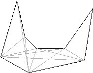
As described in previous sections, our O(n log n) algorithm does not find the optimal/shortest path. To find the optimal path, we need a tool called the visibility graph. The visibility graph of a polygon is a graph whose nodes corresponds to the vertices of the polygon, and whose edges correspond to the edges in the polygon formed by joining the vertices that can “see” each other. The figure below shows the visibility graph of the polygon.

            A Java applet computing the visibility graphs of polygons and sets of obstacles has been implemented. It can be found at http://hamp.hampshire.edu/~ppk96/cg/mApplet.html

            To compute the visibility graph of a polygon, click points on the interface and choose Compute, Visibility Graph, Polygon, Naïve Alg. This will give you the internal visibility edges. If you want the external visibility edges instead, choose Compute, Visibility Graph, Polygon, External edges, and then click one more point. You will see the external visibility edges.

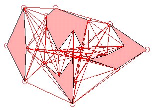
            Computing the visibility graph of a set of obstacles involves a slightly more complicated procedure. This is because you will need to tell the program which point sets define an obstacle. Moreover, you will want to have the obstacles filled with a color, so that the visibility edges will be more obvious. First, choose Compute, Visibility Graph, Obstacles, Fill Polygons. Then choose Compute, Visibility Graph, Polygon, Naïve Alg. Then click points on the interface which are the vertices of your first obstacle. After clicking all points belonging to the first obstacle, choose Compute, Visibility Graph, Polygon, Define Polygon. You will then see the first obstacle filled and bounded by a black boundary. Now you should click points that will be the vertices of the second obstacle. After you have finished, choose Compute, Visibility Graph, Polygon, Define Polygon. Again the second obstacle will be defined, and the visibility edges between the first and second obstacles will also be computed. Repeat the process for additional obstacles. If you do not want the obstacles filled, then omit the first step on Fill Polygons.
 

Why do Visibility Graphs give the shortest path?

Lemma : Any shortest path between pstart and pgoal among a set S of disjoint polygonal obstacles is a polygonal path whose inner vertices are vertices of S.

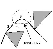
Proof by contradiction. Suppose there is a shortest path B that is not polygonal, as shown in the diagram above. We take point p on B. Since p is in the interior of the free space, there is a disc of positive radius centered at p that is completely contained in the free space. The part of B inside the disc, which is not a straight line segment, can be shortened by replacing it with a straight line connecting the two points where B enters the disc and leaves the disc. This contradicts the assumption that B is a shortest path, since any shortest path must be locally shortest, that is, any subsections of a shortest path must itself be the shortest path of that section.

            By this Lemma, the segments on a shortest path are visibility edges, except for the first and last segment. To make them visibility edges as well, we add the start and goal position as vertices to S. With this visibility graph as our road map, we can now determine the shortest path by single-source shortest path algorithms. We will return to an example of such an algorithm, Dijkstra’s algorithm, after presenting algorithms for computing visibility graphs.

Algorithms for Computing Visibility Graphs of Obstacles

Input: a set of points defining the obstacles.
Output:  a set of points which correspond to the visibility edges of the obstacles

Several algorithms exist with different time complexities.

•  O(n³) naïve algorithm – This algorithm compares every pair of points in the set of obstacles, and check if they intersect with any edges of obstacles. If a pair of points do not intersect with any edge, and that the pair is external to the obstacles, they are visibility edges. Otherwise, they are not. For a set of obstacles with n vertices in total, each vertex can pair up with (n – 1) other vertices. This will give O(n²). Each pair of points have to be compared with n edges (a set of obstacles with n vertices have n edges). This will give an O(n³) overall time complexity. This is the algorithm used in the Java applet described above.

• O(n² log n) binary search tree algorithm – This algorithm will be described in detail below.

• O(n²) algorithm using arrangements.

• O(n log n + E) algorithm, where E is the number of edges in the graph. In the worst case, E = O(n²) for a complete graph, but it is uncommon to have a complete graph. This algorithm is output-sensitive.