Week 1:

Friday

Today Ana, Faith, and I figured out how to save our Mathematica animations as animated GIF files that can be imported onto a website.

The code is actually much simpler than we expected because in Mathematica 5.0 it is possible to export a list of graphics images as a .gif type, instead of having to create each image separately and the merging them together into one animation. This is the code we used to export our Mathematica images:

Export["anim1.gif",listg,"GIF", ConversionOptions -> {"Loop" -> True}]

Here anim1.gif is the file name of the GIF animation we are creating, listg is the list of the graphics images in our animation, and "GIF" is the type of the exported file. We found that we also had to include the conversion option in which the animation loops continually (but that might not always be necessary). There are many other conversion options, which are explained in depth in the Mathematica Help Browser, under the Additional Information section at the bottom of the description of the Export method.

In order to specify where you like your export GIF animation to be saved, you can set the directory using: SetDirectory["H:"] where "H:" is the drive where the animation will be stored.

More specifically, in order to create our list of graphics to export into the GIF file, we simply appended each new image created to a list listg. We wanted the animation to pause when it had finished unfolding before looping back and beginning the animation again, so we included this conditional statement at the end of our for loop that added the last graphics image of the animation to the list eight times, to simulate this pause. This is our code for the simplest example:


listg = {}
n = 25;
For[ i = 0, i = n, i++,
  Print[i];
  t = (Pi)(i/n);
  
  g =
    Show[
      Graphics3D[
        {
          base,
          front[t],
          A[t], B[t]
        },
        Axes -> True,
        AxesLabel -> {"x", "y", "z"},
        Boxed -> False,
        PlotRange -> {{-(a + (1/2)a), a + (1/2)a}, {-1,
              b + 1}, {-1, a + (1/2)a}}
      ]
    ];
  If[i < n, listg = Append[listg,g], listg = Join[listg, {g, g, g, g, g, g, g, g}]];
]

The parts shown in purple are those that deal with the creation of a list containing the images that need to be included in the animated GIF file.


Week 2:

At the beginning of this week, we have been creating still images that will serve as figures in the teachers' guide Joe is writing. We initially decided not to change the images we had created in Mathematica, but as we were editing the document, we realized that the explainations of pop-up cards made through parallel cuts were confusing when the figures associated did not actualy show any cuts. Our pictures, as can be seen in the animation from last week, did not show any of the holes in the cards that would be created through cutting. We decided that the still images included in the document should show these white spaces in order to make the description of the cutting process clearer. This was actually a complicated change to make, because we had to calculate the points defining the holes in 3-D. For example, in the first of the series of still pictures shown below, we had to find the proportion of the length of the cut section to the length of the card in order to find the bottom two corners of the hole. The final images are much clearer than our initial attempts, so the work was worth it.

Joe also decided that it would be useful to include a few pictures of the physical pop-up cards we created as examples, so we took some digital pictures of cards as well.

Joe asked us to begin writing the section of the paper on non-paralellogram quadrilaterals, so we worked on outlining that section in the middle of the week. We had to decide which points needed to be made and the diagrams we would need to include in the explainations. As Faith had discovered the first week, there are a number of constraints that define the types of quadrilaterals that will function as pop-up cards (in other words cards that will be able to open and close completely and correctly). We decided that a good question to ask at the beginning of the section would be whether the quadrilateral could have four sides of completely different lengths, giving the following two examples:

The explaination section shows that only the picture on the right will be able to open and close completely, outlining the particular constraints.

At the end of the week, we began editing the portion of the document that Joe had written. Many of the explainations needed to be fleshed out, and we realized that one of our diagrams (showing a card that would not be able to open completely) did not make much sense in context. We decided to expand this figure so that it shows a three-image still animation, which is much clearer.


Week 3:

Wednesday

This week we are starting to work on the rotation section of the pop-up book. First we are attempting to create diagrams to explain the movement of a card created by making one perpendicular cut in the card, and then folding out the center so that a section formed by two triangles pops out. We don't have pictures to show this yet, but the geometry of this card is much more complicated than those we described in the first section. The center crease of this pop-out section actually moves along the surface of a cone, whose tip is centered at the base of the pop-out. We made a mathematica animation of this card yesterday, but today we discovered that everything we did was actually wrong because the cone we were tracing was centered across the card crease, when it should actually be centered around the line that bisects the right angle between the card crease and the line perpendicular to this (parallel to the card base), formed when the pop-up card is completely closed. We have had a lot of trouble calculating the correct points to create this new animation, and do not have a good diagram of it yet.


Thursday


Today we were able to finish our animation because Joe worked on it some at home, fixing the part that we didn't know how to complete. Once the circles displaying the cone were working, we were able to add the card and the polygons that pop out of the card pretty easily. There were a few complications because it turns out the equations used to find the points on the pop-out section can not be solved for the angle 0 or pi, so we could not include the completely open or completely closed view in our animation.


Friday


We decided that we will next need to explain the concept of moving the fold-out section of the v-fold rotation card away from the center of the card, pointing out that the motion created by the card is exactly the same. This was a bit complicated because we had to use two separate angles--the angle formed by the card and the angle between the fold-out and the card base--to calculate the points needed.

Today we also learned a little a little about how to use POV-Ray, which we will be using to make a diagram showing that the intersection of a cone and a sphere is a circle.


Week 4:

Monday

This week we are starting to work in POV-Ray a little bit, experimenting with ways that we can create a good image displaying that the intersection of a sphere and a cone is a circle. We have figured out how to use the program on a basic level, enough so that we can make a transparent sphere (use the glass.inc package and choose a glass color). We have discovered that is actually difficult to design a clear image that displays this point though. In order to see the circle that is created, a camera must look at the cone dead on, but this is confusing because it does not really look like a cone. So we are still working on finding the optimal view.


Tuesday

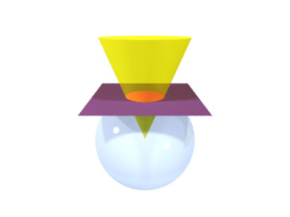
Today we finished our POV-ray figure of the cone intersecting the sphere. It came out pretty well, but we also learned a lot more about what can actually be accomplished in POV-ray, which made our accomplishment seem much less significant. We had some difficulties with getting the camera and the obejcts in the right place to create the picture we wanted. What we learned is that the coordinate system in POV-ray is very counter-intuitive, and that it is much easier to move your objects around the "world" than to move the camera so that it provides the desired view of the objects. The camera angle can be modified in many ways, but it is much harder to do this than to move the objects themselves. We also had some trouble getting the lighting to do what we wanted, because we were using simple spot lights which create a lot of contrast and strong shadows. This made our diagram a little hard to understand, so we ended up using so radiosity lighting that Joe had designed for another project, which looks much better. This is the code we used to create the lighting:

#declare RAD = on;

global_settings {
  #if(RAD)
      radiosity { 
        
      pretrace_start 0.08
      pretrace_end   0.04
      count 35

      nearest_count 5
      error_bound 1.8
      recursion_limit 3

      low_error_factor 0.5
      gray_threshold 0.0
      minimum_reuse 0.015
      brightness 1

      adc_bailout 0.01/2
    }//radiosity
  
  #end //if
}//global settings
	  

We also used a few area lights, which produce softer shadows.

In order to create a sharp final image, we had to figure out how to use antialiasing in POV-ray. After doing a little searching around in the help menu, we found that you can manipulate antialiasing through the INI file settings. When you choose the Ini run setting, POV-ray gives you a number of options, including a command line where you can include different settings. In order to specify antialiasing, you can type either Antialias_Threshold=n.n or +An.n where n.n is a number between 0 and 1, which determines the level of antialiasing. n = 0.0 gives the highest quality. We discovered that you cannot just set n equal to 0, but must use the real number 0.0 in order for it to work. After all of this work, we also realized that the drop down menu of image rendering sizes that appears at the top left of the POV-ray screen allows you to select sizes with or without antialiasing, which allows you to turn antialiasing on without all of this work (although understanding how to manipulate the Ini settings is useful and gives you more control).


Wednesday

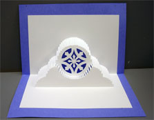
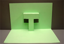
This morning I finished an example card I was making to show how v-folds can be used in the more artistic sort of card design that will be more often seen by children. It uses a sigle cut, creating two v-folds (one above the cut and one below it) to form the mouth of a bird. We will be taking pictures of this and a few other example cards later this week I think.

This afternoon we made a few quick diagrams for the document, and then worked on figuring out how to create animations with POV-ray. It turns out that it was not actually that difficult to do. We decided to practice animations by rotating the image of the intersection of the sphere and the cone we created yesterday 360 degrees in the plane orthogonal to the x axis. This produced an animation that shows the top and bottom views of the objects, which can make the circle of intersection clearer. In order to create this animation, we first created a union of all of the objects we wanted to rotate using the union command. Before closing the union, we used a rotate command to determine how we wanted the objects to move during our animation: rotate<-clock*360,0,0>. In order to create an animation, you must use the built-in clock variable somewhere in your code to determine the movement of your objects over time. There is a pretty good description of the variable if you search for "clock" in the help menu, but in order to understand this it is useful to first look at the INI options you must include for animations. If you select the Ini play option, above the command line there is a button allowing you to edit the specified INI settings. If you click on this, a window will open showing you the code that determines the settings for each size. You can change these settings to allow the creation of more than one image when you render your code. To do this, first find the setting you would like to use in the INI code. For example, for each image size there is a block of code that looks like this:

	[160x120, No AA]
    Width=160
    Height=120
    Antialias=Off    

It specifies the image size and whether or not there will be antialiasing (AA). Find the block of code indicating the options you want to use for your animation. At the end of the code, add two new lines

   Initial_Frame = 1 
   Final_Frame = 5

These new line specify the number of frames that you will to produce when you run your code. Here, we will create 5 separate images. The number of frames can be changed as desired. This relates to the clock variable, because clock represents a number between 0 and 1which is determined by the number of frames that you are using. This is a really nice feature, because POV-ray will divide the clock variable evenly between each of your frames, so that it increases at an even rate for each image you create. This means that when we rotated our objects by -clock*360 degrees in the x direction, our image was rotated by a different portion of the whole angle each time, creating a smooth animation.

In POV-ray, unfortunately, you cannot export a series of images into a GIF file the way you can on Mathematica. In order to string our individual BMP files into a GIF animation, we had to use outside software. I found a program with a free 30 day trial online that is pretty easy to use, called GIF Movie Gear. All I had to do was choose the "insert frames" option and import all of the BMP images that I wanted to include in the animation. The program does the rest--all you have to do is hit the play button and you can see your animation. We're going to try to play around with the software a bit over the next few days, to see if it is worth buying the real version, which costs about $40. We are also thinking about trying to create a POV-ray animation in an MPEG file, which would have much better quality, but is not quite as web-compatible. We'll have to see.


Thursday

click here to animate


Today we decided that there were a number of ways that our animation could be improved, so we modified it a bit, changing the colors and dimensions to better prove our point. The final product is looking pretty nice. Did I mention that I love POV-ray?

Next we started working on an animation that will display the intersection of the cone with the median plane of a rotary motion pop-up card. Didn't get too far.


Friday

Today we worked on the median plane animation in POV-ray, and had a lot of difficulty describing the creation of the circle that traces the intersection of the median plane and the cone. What we want our animation to show is that as the median plane moves through the cone defined by the rotary motion of the v-fold, the intersection is a quarter-circle (or wedge, if you look at the entire intersection). In order to animate this in POV-ray, we must use the intersection of a thin torus and a wedge-shaped prism to draw something that looks like a portion of a circle on the median plane. This coordinates of the wedge were a little tricky to find, but our main problem now is that we cannot find the angle that determines how much of the circle should be drawn at each point in time. Initially, we thought that the quarter circle would be drawn at a constant rate, but it appears that this is not actually true. We cannot see how the rate of change of this anlge relates to anything else in our scenario, so we haven't yet been able to produce an accurate animation.


Week 5:

Tuesday

Over the past two days we have been working on our median plane animation. In the meantime, Joe found some problems with the v-fold animations that we did last week. It turns out that the point we were using as the center of the v-fold was actually incorrect. We had to do some complicated calculations to fix it, but it wasn't too hard once we figured out what we had to change. These are the new animations:

Once we had fixed this problem, we went back to our work on the median plane animation. We proved to ourselves that the half-circle drawn by the median plane intersecting the cone is not created at a constant rate, and the angle definetly does not grow at the same rate as the median plane angle. We did not know how to figure out how this new angle relates to the rest of our card, so we decided to use mathematica to calculate the angles that we would need to create our animation. This turned out to be a little bit more difficult than we expected. Joe helped us by drawing a vector in our mathematica animation that lay in the median plane, and then calculated the angle between this vector an the vector tracing the rib of the cone. This is the angle we needed for our POV-ray animation. to be continued...